See also
interpretation technologies
rock physics
computer mapping
well to seismic ties
Some examples of Time to Depth Conversion studies.
|
|
See also Some examples of Time to Depth Conversion studies. |
||
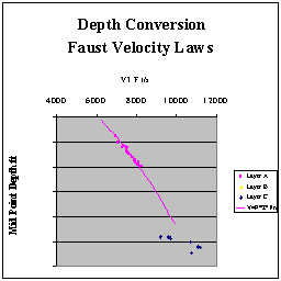
| Following an analysis of 60 wells, depth conversion down through the first and deeper layers was undertaken using the Faust Power Law:
V = F. Z 1/N Z= the depth from the surface F= a factor depending on the lithology and age of the sequence. This exponential relationship of interval velocity to depth was used so as not to unrealistically increase the velocity when the function is projected beyond the well penetration limit. |
Velocity Study Exponential increase of velocity with depth of burial [Faust Law]. |
|
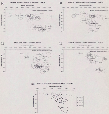
A study of 28 wells in a Tertiary reservoir. Here the aim was to see if there was a relationship with a layer's velocity and its thickness, for 4 seperate reservoir zones. A 3rd dimension is added to the graph by making the symbol proportional to the layer's N/G. While there is a general increase of Interval Velocity with thickness, (the deposition is thought to be channel controlled with the higher velocity sands concentrated in the channels) there is too much of a spread of values to provide an accurate depth conversion function. |
Velocity Study Investigating variation of velocity to thickness and N/G. |
||
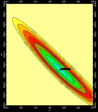
The examples 1 & 2 above show how I look to model the mean interval velocity of the layer velocity in terms of depth of burial or thickness. A similar approach would be to look at the behaviour of the Instantaneous Velocity of a layer. Vins = Vo + KZ, describing the instantaneous velocity behaviour as a function of depth. The function can be derived from one or more wells [sonic data]. Vertical lithological changes within the layer influence this function strongly as well as burial effects. The K in this function is sometimes referred to as "instantaneous K". |
|||
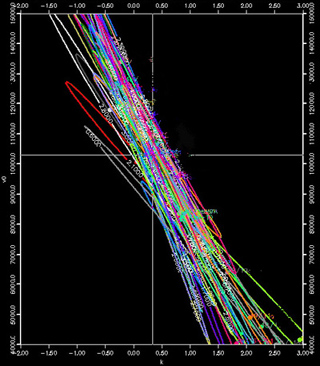
Dr Al-Chalabi has shown that the Vo, K parameters have a non-uniqueness if you accept a margin of error inherent in the measurements. This non-uniqueness leads to a solution trough where Vo,K combinations can tie the well equally well. Graph A is an output from Velit of one such solution trough for a Triassic layer in the UK's Southern Gas Basin. The Velit program has been used to provide a robust calculation of V0,K solution troughs for several wells.The overlap of the solution troughs suggests that the velocity behaviour should be explained by a variable Vo, while a constant K could tie all the wells with equal accuracy. |
Graph A V0,k solution trough for one well. |
Graph B Overlap of solution troughs |
|